G²ARD-GS: Geometry-Guided Anchor-Regularized Gaussian Splatting Distillation

A geometry-guided distillation framework for compact 3D Gaussian maps

Fixed-budget 10x comparison of ground truth, PUP, NanoGS, and G²ARD-GS across two held-out views and one training view

Matched-budget MatrixCity reconstructions on two held-out views and one training view. PUP, NanoGS, and G²ARD-GS use the same 10× Gaussian budget and camera poses.

Abstract

Dense colored LiDAR maps provide accurate city-scale geometry, but their massive point counts make storage, transmission, rendering, and adaptation costly. Although 3D Gaussian Splatting (3DGS) enables photorealistic real-time rendering, directly converting dense maps into Gaussian representations retains much of this primitive burden, while aggressive compression can remove the local surface support required for stable novel-view synthesis and downstream geometric tasks. We introduce G²ARD-GS, a geometry-guided distillation framework that compresses dense LiDAR-assisted Gaussian models while preserving their geometric structure for subsequent reuse. G²ARD-GS employs a multi-round simplify-and-distill process: geometry-aware simplification preserves locally distinctive surface structures, while anchor-regularized recovery optimizes a fixed-topology student with the standard 3DGS renderer, without densification or pruning. Geometry-aware informative-view selection further provides complementary supervision under a limited view budget. On MatrixCity, G²ARD-GS achieves the best PSNR, SSIM, and LPIPS across matched 5×–30× compression budgets, outperforming PUP by 3.2–6.8 dB in PSNR. Its frozen geometry also improves off-trajectory appearance adaptation by 3.7–4.9 dB over PUP 3D-GS and preserves image-to-model registration accuracy on Cambridge KingsCollege under 30× compression.

Method

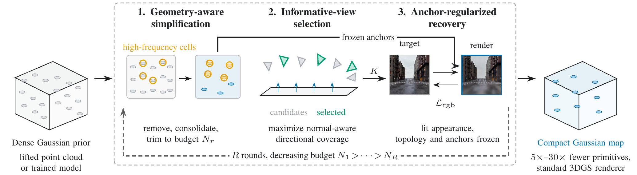
G²ARD-GS pipeline: geometry-aware simplification, informative-view selection, and anchor-regularized recovery repeated over rounds of decreasing budget

G²ARD-GS distills a dense Gaussian prior — either a lifted point cloud or a trained model — into a compact student through a multi-round simplify-and-distill loop: (1) geometry-aware simplification trims toward the next primitive budget while protecting high-frequency surface structure and freezing construction-time anchors; (2) informative-view selection spends a limited supervision budget on the views that best observe the scene's surfaces; and (3) anchor-regularized recovery refits appearance on a fixed topology, using the standard 3DGS renderer with no densification or pruning. Repeating this over rounds of decreasing budget yields a 5×–30× smaller model in the standard 3DGS representation.

Results

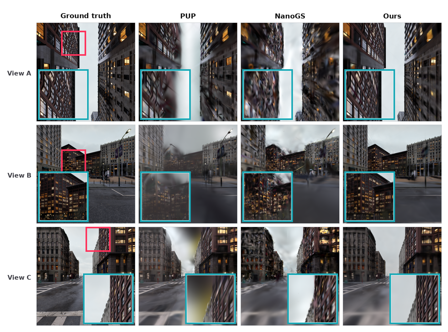
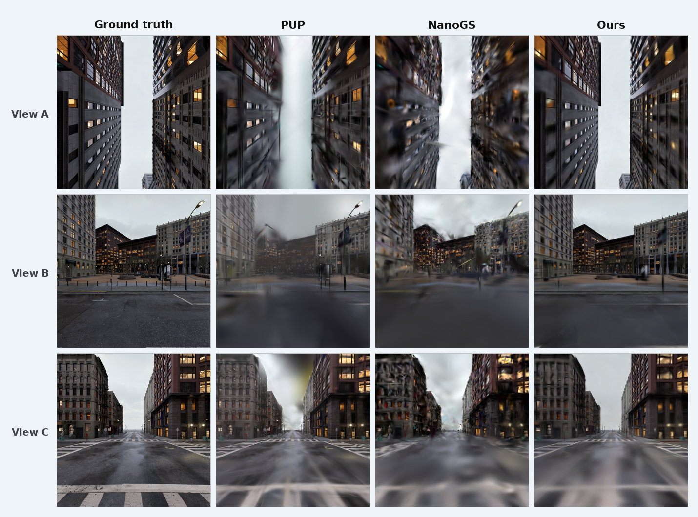
Three-view 10x reconstruction comparison using train view 1434 and val views 459 and 445

Fixed 10× budget — View A = train 1434, View B = val 459, and View C = val 445. Picture-in-picture crops use identical coordinates across methods; A/B place the enlargement at lower left and C at lower right. Bright boxes in the Ground truth column mark each crop source.

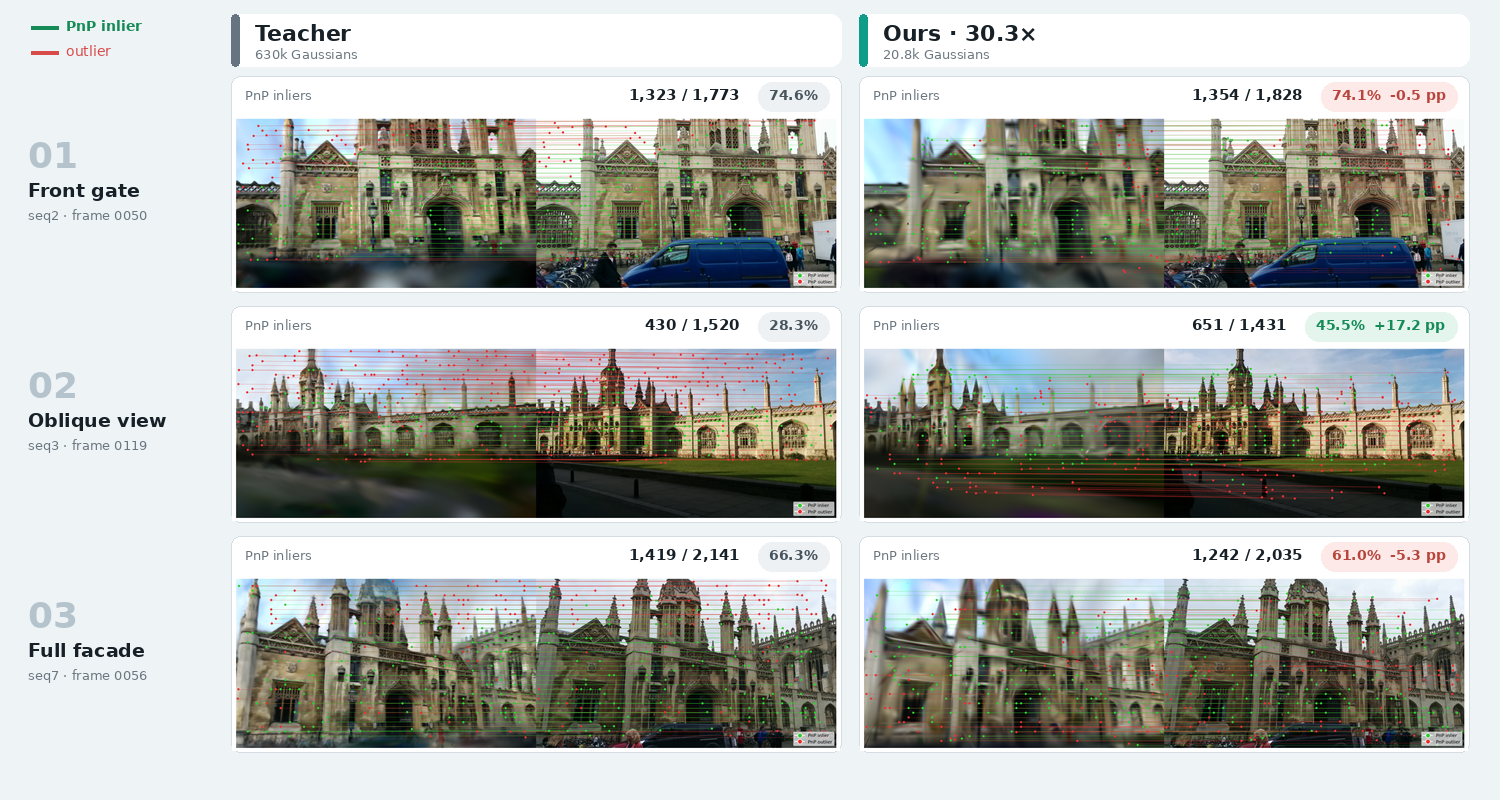
Three selected-view GS-CPR registration comparisons between the 630k teacher and the 30.3x compressed 20.8k-Gaussian model

GS-CPR on three selected KingsCollege frames — green lines are PnP inliers and red lines are outliers. Relative to the 630k teacher, the 20.8k-Gaussian model is 0.5 pp lower on the front gate, 17.2 pp higher on the oblique view, and 5.3 pp lower on the full facade. Click the figure for full resolution.

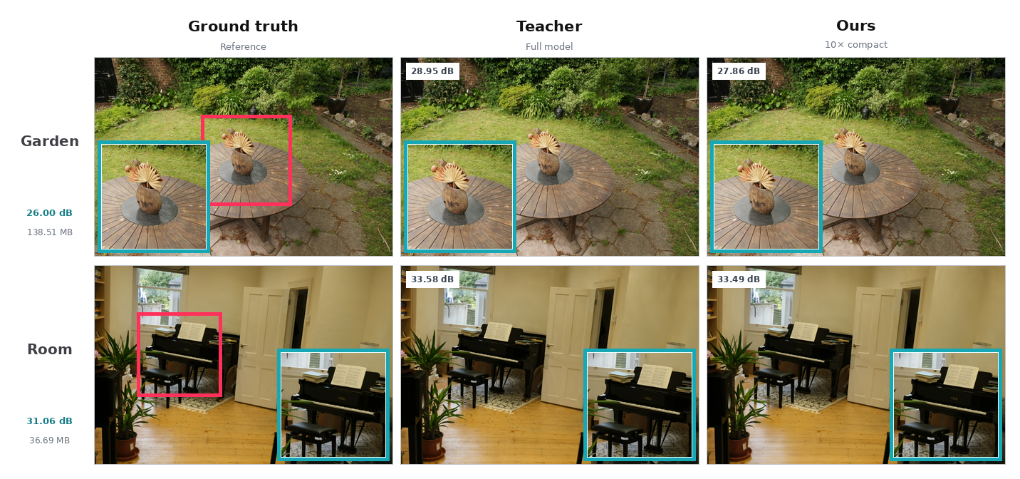
Mip-NeRF 360 Garden and Room comparisons with matched picture-in-picture detail crops for ground truth, teacher, and our 10x compact model

Mip-NeRF 360 at 10× — Garden and Room use matched crop coordinates across Ground truth, Teacher, and Ours. Pink boxes mark the crop source on Ground truth; cyan picture-in-picture panels show the same high-frequency region. The compact files are 138.51 MB and 36.69 MB, respectively. Click the figure for full resolution.

Video Results

Continuous novel-view renderings from our compact students, played back along every camera pose of each scene. All three use the same frozen 10× recipe with no per-scene tuning.

MatrixCity block_A — street-level flythrough of the 10× student distilled from a 5.99M-Gaussian prior. A 40 s excerpt of the full 4,075-view trajectory.

Mip-NeRF 360 — Garden — all 185 views of the 10× student (586,886 Gaussians, 138.51 MB).

Mip-NeRF 360 — Room — all 311 views of the 10× student (155,457 Gaussians, 36.69 MB).

Quantitative Results

Table 1 — Compression-ratio sweep

MatrixCity block_A, dense geometric prior 5,989,675 Gaussians, 510 in-distribution held-out views. Every row is re-evaluated with the same gsplat renderer and float Alex-LPIPS protocol.

Ratio	Method	Size (MB) ↓	PSNR ↑	SSIM ↑	LPIPS ↓
5×	PUP	297.09	17.41	0.666	0.518
	LightGaussian	297.09	14.04	0.554	0.812
	NanoGS	297.09	20.08	0.658	0.545
	Ours	283.01	24.20	0.763	0.409
10×	PUP	148.55	18.27	0.673	0.531
	LightGaussian	148.55	14.25	0.562	0.822
	NanoGS	148.55	18.52	0.620	0.640
	Ours	141.65	22.78	0.727	0.469
20×	PUP	74.27	18.12	0.656	0.565
	LightGaussian	74.27	13.99	0.553	0.827
	NanoGS	74.27	17.35	0.600	0.706
	Ours	70.98	21.72	0.696	0.532
30×	PUP	49.02	17.99	0.645	0.588
	LightGaussian	49.02	13.40	0.531	0.834
	NanoGS	49.02	16.89	0.593	0.730
	Ours	47.42	21.21	0.680	0.567

Table 2 — Geometric-base reusability

Geometry is frozen while appearance is refit on 341 driving views. OOD metrics use a disjoint 495-view split; Adapt PSNR uses the remaining 49 trajectory views.

Ratio	Method	Size (MB) ↓	OOD PSNR ↑	OOD SSIM ↑	OOD LPIPS ↓	Adapt PSNR ↑
10×	Ours	141.39	21.38	0.718	0.461	26.40
	PUP	141.39	16.45	0.652	0.538	21.60
	LightGaussian	141.39	14.86	0.577	0.773	13.91
30×	Ours	47.15	20.17	0.675	0.552	24.34
	PUP	46.68	16.49	0.633	0.589	21.10
	LightGaussian^†	46.68	13.60	0.542	0.805	12.19

^† LightGaussian 30× has 11 all-black OOD renders; its aggregate excludes those failures and uses 484 views.

Table 3 — GS-CPR registration

KingsCollege, 343 test frames, with the same ACE coarse initialization for the teacher and every compact model.

Metric	Teacher 630k	Ours 5× 126k	Ours 10× 63.0k	Ours 20× 31.5k	Ours 30.3× 20.8k
Size (MB) ↓	148.91	29.88	15.00	7.56	5.03
Accuracy @ 10 cm / 5° ↑	17.5%	18.7%	22.2%	17.2%	18.4%
Accuracy @ 5 cm / 5° ↑	2.9%	5.0%	5.5%	4.4%	5.0%
Accuracy @ 2 cm / 2° ↑	0.9%	0.6%	0.0%	0.0%	0.0%
Median translation ↓	27.0 cm	23.9 cm	22.6 cm	22.7 cm	22.4 cm
Median rotation ↓	0.39°	0.36°	0.33°	0.34°	0.36°
Mean translation ↓	39.9 m	9.1 m	10.1 m	11.5 m	12.3 m
Mean rotation ↓	15.8°	13.6°	12.8°	12.3°	13.8°

Table 4 — Mip-NeRF 360 evaluation

INRIA evaluation with LPIPS-VGG and llffhold=8. Sizes are measured from the canonical PLY files used for evaluation.

Scene	Model	Gaussians	Size (MB) ↓	PSNR ↑	SSIM ↑	LPIPS ↓
Garden	Teacher	5,868,851	1,455.48	27.39	0.867	0.107
Garden	Ours 10×	586,886	138.51	26.00	0.771	0.266
Room	Teacher	1,554,566	385.53	31.37	0.919	0.218
Room	Ours 10×	155,457	36.69	31.06	0.892	0.285

Size is the native serialized Gaussian model file in decimal MB (bytes / 1,000,000); optimizer state, logs, renders, and camera files are excluded. Table 1 uses each method's native evaluation artifact (.ply for baselines, .pt for ours); Tables 2–3 use .pt checkpoints.

BibTeX

@misc{g2ardgs,
  title  = {G$^2$ARD-GS: Geometry-Guided Anchor-Regularized Gaussian Splatting Distillation},
  year   = {2026},
  url    = {https://github.com/Patrick1159/gard-gs}
}